Mapping the seabed
A simulated study: an image of the seabed, from a single beam of sound.
Date: 2020, finished in 2026
How to draw from a single-beam sonar the most faithful image of a seabed, and read its relief and its nature? Another TIPE subject, considered in the preparatory classes in 2020, on the same “Ocean” theme: little explored then, with a few devices drawn to aim the transducer.
In 2026 I decided to see it through, as a study and a simulation: a transducer fixed in a sealed sphere turned by three wheels, an inertial unit to know where the beam points, a line-by-line sweep, and the image rebuilt sharper than the beam, by deconvolution. The piloting program is written, the code of the two boards too; the whole drives a simulated rig, over a simulated 50 × 50 cm bed. A 58-page report accounts for it, to read from this page.
Nothing is built yet: every result on this page is a simulation, and the report says so.
The result
What was done
01
The simulation of the bed and the echoes
A relief on a 2 mm grid with four bed types, and for each pulse the synthesised echo: the transducer’s directivity, the sonar equation, backscatter against the angle, speckle noise.
Python · NumPy · SciPy
02
The sphere and its cradle
The device’s geometry: the three wheels 35.26° from the pole for perpendicular axles, the buoyancy that presses the sphere against them, the transmissible torques, the magnetic couplings.
03
The piloting
The line-by-line sweep, the 100 Hz control and the orientation estimate from the inertial unit, with the reset at every stop; one program for the simulated rig and the real one.
Python
04
Electronics and firmware
The transmit and receive chain, and the code of two boards: one in the sphere, for the pulse, the echo’s digitisation, the inertial unit and the optical link; the other on the cradle, for the motors. Never compiled for the boards: only the shared part is tested on a computer.
C++ · Raspberry Pi Pico
05
Imaging and classification
The relief from the echoes’ barycentre, then by deconvolution over angles and range; the bed’s nature cell by cell, from five positions.
Python · Richardson–Lucy
06
The report
Fifty-eight pages, begun in 2020 and finished in 2026, with the programs in the appendix and twenty-one tests that check the physics and the system.
LaTeX · unittest
How it works
Scroll: the drawing follows.
01 / 07
Mapping a seabed with a single beam
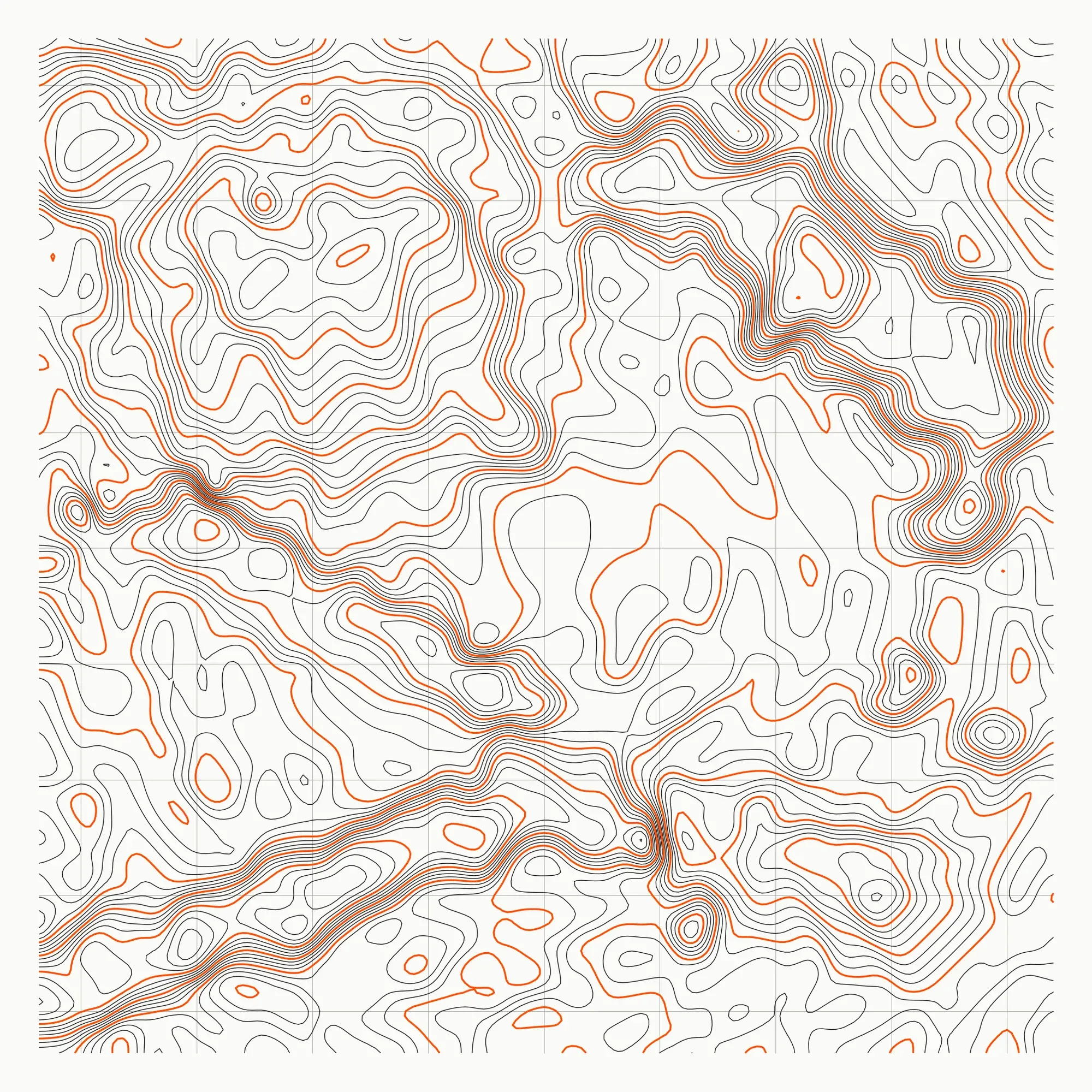
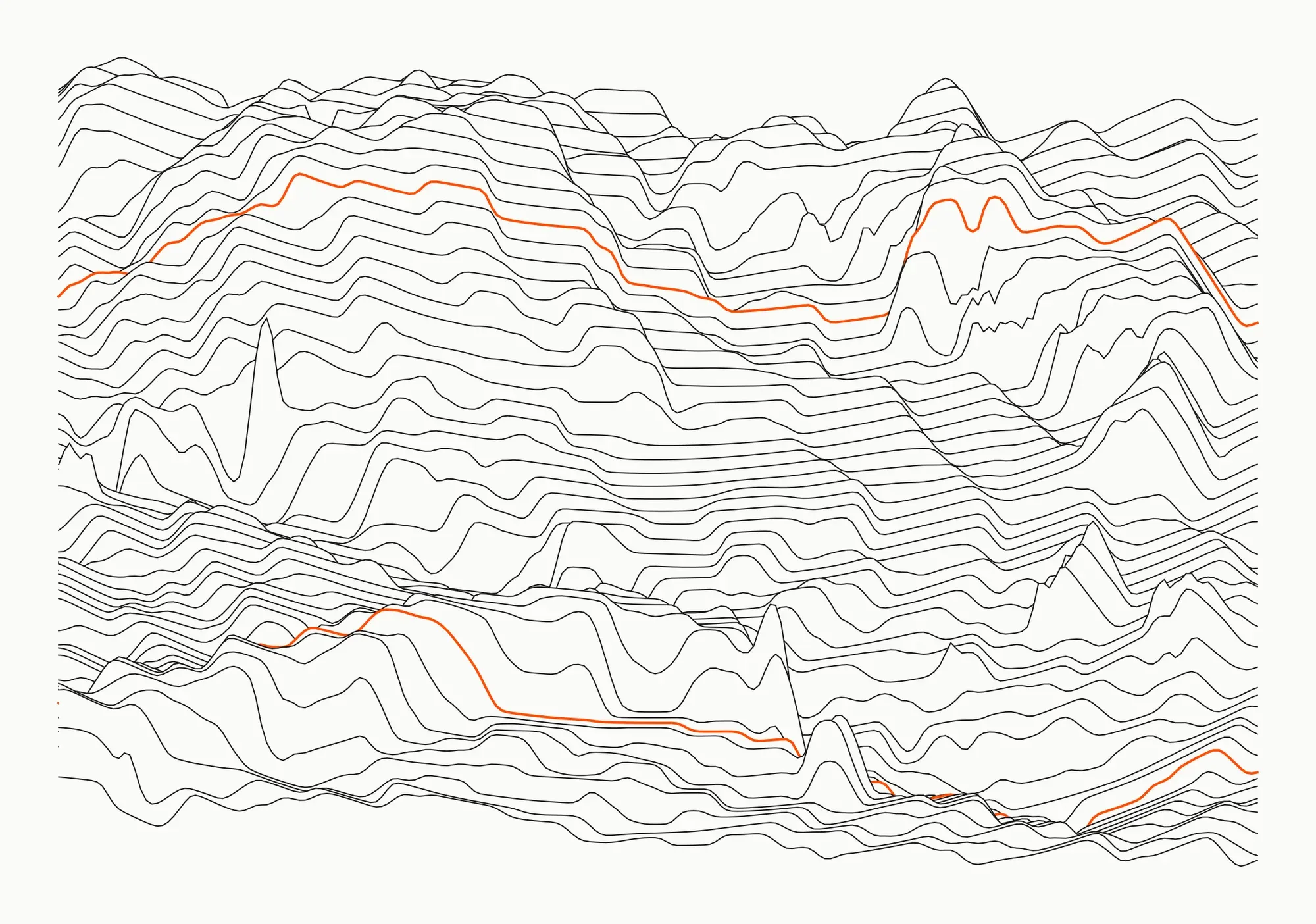
Draw from a single-beam sonar the most faithful image of a seabed, and read its relief and its nature. The bed is simulated, 50 × 50 cm: a mound, a hollow, sand ripples, a silted channel, five rocks, a buried pipe, a wreck, over four bed types, sand, gravel, mud and rock. Nothing is built: everything here is simulated.
02 / 07
Send a pulse, wait for the echo
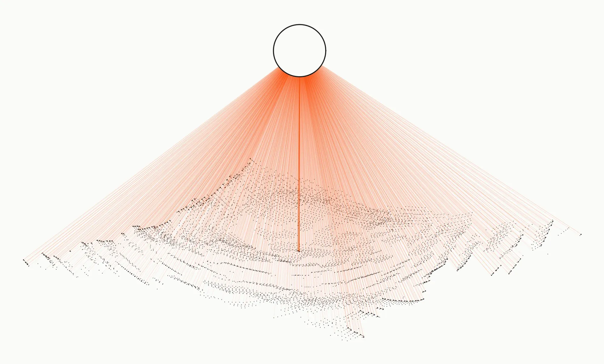
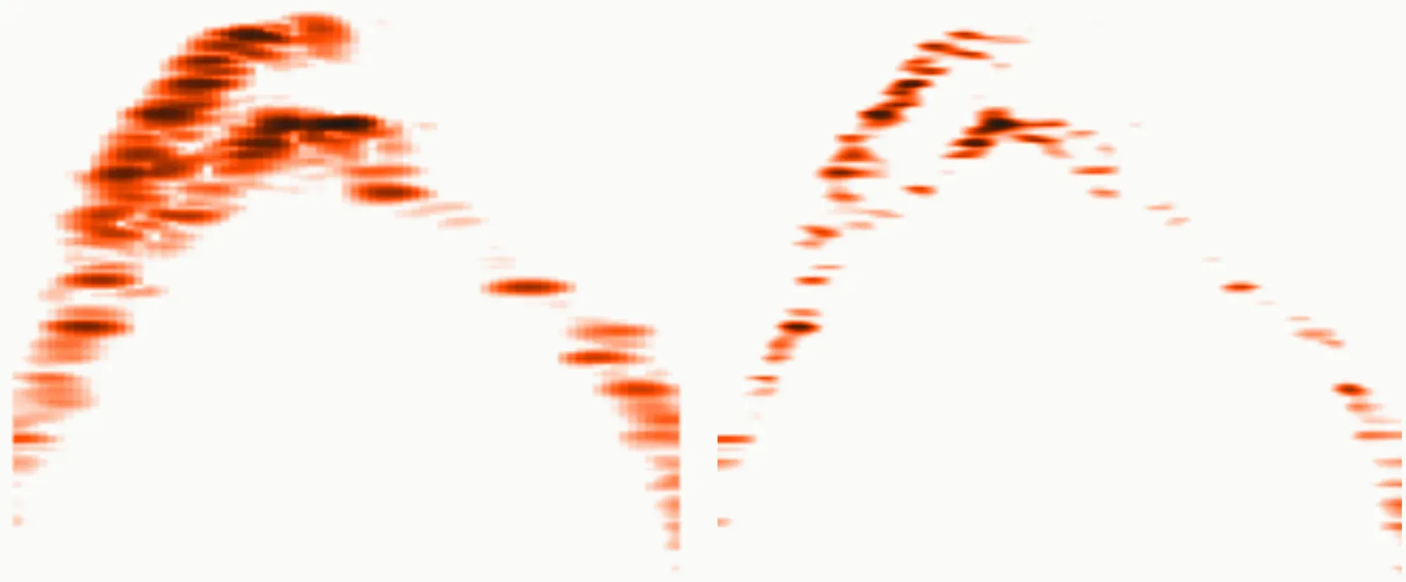
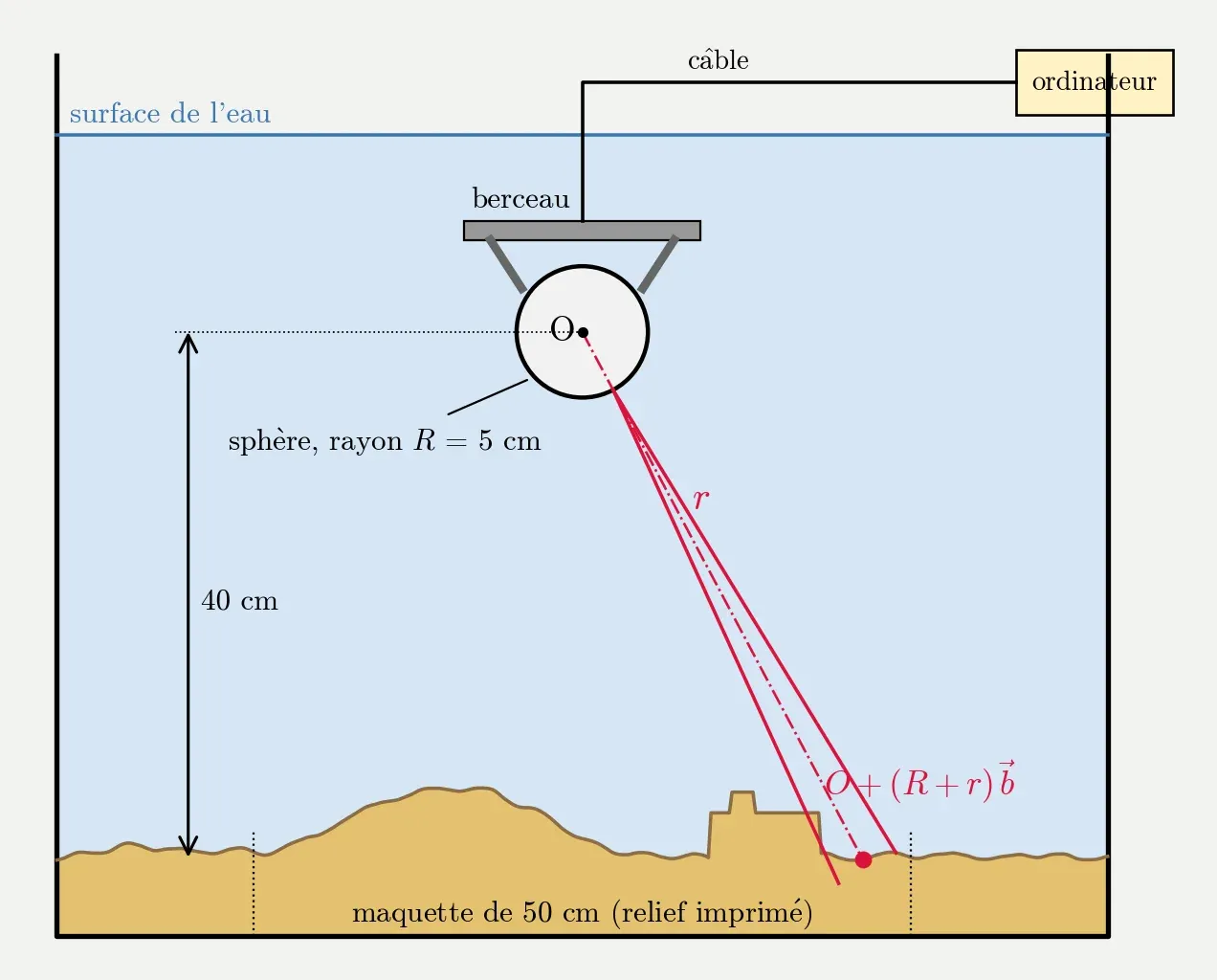
A 12.7 mm piezoelectric disc emits five periods near 1 MHz, then listens. The time the echo takes to come back gives the distance, in the beam’s direction, seven degrees wide: at 35 cm it lights a spot of four centimetres. The shape and strength of the echo also tell what the bed is made of: seen obliquely, mud returns twenty to thirty decibels less than rock.
03 / 07
A sphere turned by three wheels
The transducer is glued at the south pole of a sealed 10 cm sphere, immersed. Its buoyancy presses it against three omnidirectional wheels, set 35° from the pole so that their axles are perpendicular, like the three edges of a cube’s corner; each motor, in its sealed box, drives it through a magnetic coupling. Every beam leaves from its centre, which never moves.
04 / 07
Know where the beam points
An inertial unit at the sphere’s centre gives its orientation, two hundred times a second. Every time the three motors stop, the drift of its gyros is measured again. A board inside the sphere times the pulse, digitises the echo and talks to the cradle through an optical link across the wall; a second one, on the cradle, drives the motors. In simulation, the aim is off by 0.22° on average.
05 / 07
Sweep the bed, line by line
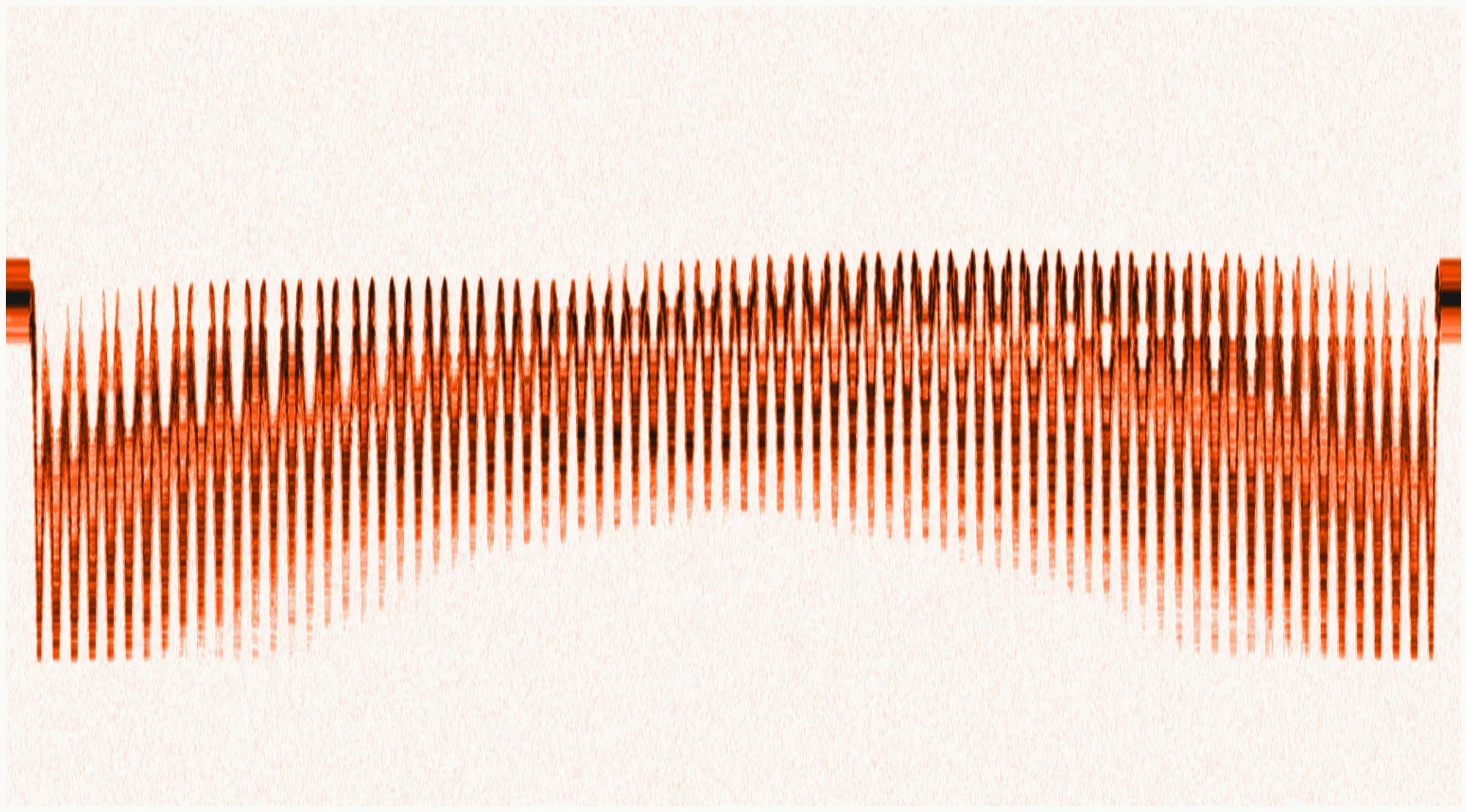
The sphere sweeps a ±38° square, line by line, back and forth, one pulse per degree: 8,333 pulses in 166 seconds. The piloting program is the real one; here it drives a simulated rig, with its slips, its delays and its lost messages.
06 / 07
Rebuild the relief, sharper than the beam
The beam blurs the bed, like a photograph out of focus: each point is seen by about twenty pulses. The classical method places the barycentre of each echo on the beam’s axis and strays from the true relief by 9.8 mm; by treating all the pulses together, through deconvolution over angles and range, the error drops to 7.5 mm, in simulation.
07 / 07
Recognise the bed’s nature
The echo’s strength against the viewing angle betrays the bed. From five positions of the sphere, each three-centimetre cell is compared with the curves of the four types, and gets the nearest: 64 % of cells right on average, against 25 % by chance. Reliable at the scale of zones, not of the spot.
Specifications
- Date
- 2020, finished in 2026
- Context
- A personal scientific project, begun in preparatory classes as a TIPE research project, that I wanted to carry on and finish.
- Built with
- Python (NumPy, SciPy, Matplotlib) · C++ for Raspberry Pi Pico · LaTeX